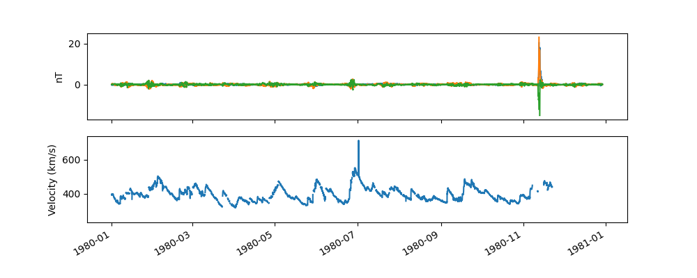
Voyager

Plotting Voyager magnetic field and plasma data.

Import the required packages

from heliopy.data import voyager
from datetime import datetime
import matplotlib.pyplot as plt

Download and load the merged dataset for a single year

starttime = datetime(1980, 1, 1)
endtime = datetime(1980, 12, 30)
data = voyager.voyager1_merged(starttime, endtime)
print(data.columns)

Out:

Downloading VOYAGER1_COHO1HR_MERGED_MAG_PLASMA for interval 1980-01-01 00:00:00 - 1981-01-01 00:00:00

0it [00:00, ?it/s]
3193it [00:00, 44907.38it/s]
['heliocentricDistance', 'heliographicLatitude', 'heliographicLongitude', 'ABS_B', 'F', 'BR', 'BT', 'BN', 'V', 'elevAngle', 'azimuthAngle', 'protonDensity', 'protonTemp', 'protonFlux1_LECP', 'protonFlux2_LECP', 'protonFlux3_LECP', 'protonFlux1_CRS', 'protonFlux2_CRS', 'protonFlux3_CRS', 'protonFlux4_CRS', 'protonFlux5_CRS', 'protonFlux6_CRS', 'protonFlux7_CRS', 'protonFlux8_CRS', 'protonFlux9_CRS', 'protonFlux10_CRS', 'protonFlux11_CRS', 'protonFlux12_CRS', 'protonFlux13_CRS', 'protonFlux14_CRS', 'protonFlux15_CRS', 'br_uncertainty', 'bt_uncertainty', 'bn_uncertainty']

Plot the data

fig, axs = plt.subplots(nrows=2, figsize=(10, 4), sharex=True)

ax = axs[0]
for var in ['BR', 'BT', 'BN']:
    ax.plot(data.index, data.quantity(var), label=var)
ax.set_ylabel('nT')

ax = axs[1]
ax.plot(data.index, data.quantity('V'))
ax.set_ylabel('Velocity (km/s)')

fig.autofmt_xdate()
plt.show()