
Note
Click here to download the full example code
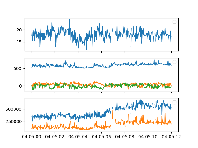
A short example showing how to import and plot plasma data.
Out:
Creating new directory /home/docs/heliopy/data/helios/E1_experiment/New_proton_corefit_data_2017/ascii/helios2/1976
Downloading http://helios-data.ssl.berkeley.edu/data/E1_experiment/New_proton_corefit_data_2017/ascii/helios2/1976/h2_1976_096_corefit.csv


Index(['B instrument', 'Bx', 'By', 'Bz', 'sigma B', 'Ion instrument', 'Status',
       'Tp_par', 'Tp_perp', 'carrot', 'r_sun', 'clat', 'clong',
       'earth_he_angle', 'n_p', 'vp_x', 'vp_y', 'vp_z', 'vth_p_par',
       'vth_p_perp'],
      dtype='object')
from datetime import datetime, timedelta
import heliopy.data.helios as helios
import matplotlib.pyplot as plt

starttime = datetime(1976, 4, 5, 0, 0, 0)
endtime = starttime + timedelta(hours=12)
probe = '2'

corefit = helios.corefit(probe, starttime, endtime)

print(corefit.data.keys())

fig, axs = plt.subplots(3, 1, sharex=True)
axs[0].plot(corefit.data['n_p'])
axs[1].plot(corefit.data['vp_x'])
axs[1].plot(corefit.data['vp_y'])
axs[1].plot(corefit.data['vp_z'])
axs[2].plot(corefit.data['Tp_perp'])
axs[2].plot(corefit.data['Tp_par'])

for ax in axs:
    ax.legend()
plt.show()
Total running time of the script: ( 0 minutes 0.980 seconds)