
Note
Click here to download the full example code
How to plot orbits from SPICE kernels.
In this example we download the Parker Solar Probe SPICE kernel, and plot its orbit for the first year.
import heliopy.data.spice as spicedata
import heliopy.spice as spice
from datetime import datetime, timedelta
import astropy.units as u
import numpy as np
Load the solar orbiter spice kernel. HelioPy will automatically fetch the latest kernel
kernels = spicedata.get_kernel('psp')
kernels += spicedata.get_kernel('psp_pred')
spice.furnish(kernels)
psp = spice.Trajectory('SPP')
Out:
Downloading https://sppgway.jhuapl.edu/MOC/reconstructed_ephemeris/2018/spp_recon_20180812_20181008_v001.bsp
Downloading https://sppgway.jhuapl.edu/MOC/reconstructed_ephemeris/2018/spp_recon_20181008_20190120_v001.bsp
Downloading https://sppgway.jhuapl.edu/MOC/reconstructed_ephemeris/2019/spp_recon_20190120_20190416_v001.bsp
Downloading https://sppgway.jhuapl.edu/MOC/ephemeris//spp_nom_20180812_20250831_v035_RO2.bsp
Downloading https://naif.jpl.nasa.gov/pub/naif/generic_kernels/lsk/naif0012.tls
Downloading https://naif.jpl.nasa.gov/pub/naif/generic_kernels/spk/planets/de430.bsp
Downloading https://naif.jpl.nasa.gov/pub/naif/generic_kernels/pck/pck00010.tpc
Downloading https://naif.jpl.nasa.gov/pub/naif/pds/data/nh-j_p_ss-spice-6-v1.0/nhsp_1000/data/fk/heliospheric_v004u.tf
Generate a time for every day between starttime and endtime
starttime = datetime(2018, 8, 14)
endtime = starttime + timedelta(days=365)
times = []
while starttime < endtime:
    times.append(starttime)
    starttime += timedelta(hours=6)
Generate positions
psp.generate_positions(times, 'Sun', 'ECLIPJ2000')
psp.change_units(u.au)
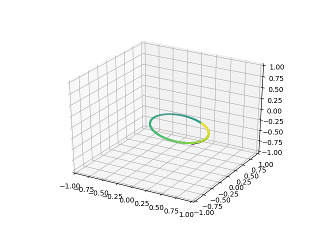
Plot the orbit. The orbit is plotted in 3D
import matplotlib.pyplot as plt
from mpl_toolkits.mplot3d import Axes3D
from astropy.visualization import quantity_support
quantity_support()

# Generate a set of timestamps to color the orbits by
times_float = [(t - psp.times[0]).total_seconds() for t in psp.times]
fig = plt.figure()
ax = fig.add_subplot(111, projection='3d')
kwargs = {'s': 3, 'c': times_float}
ax.scatter(psp.x, psp.y, psp.z, **kwargs)
ax.set_xlim(-1, 1)
ax.set_ylim(-1, 1)
ax.set_zlim(-1, 1)
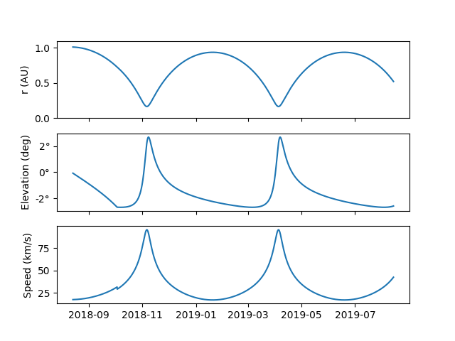
Plot radial distance and elevation as a function of time
elevation = np.rad2deg(np.arcsin(psp.z / psp.r))

fig, axs = plt.subplots(3, 1, sharex=True)
axs[0].plot(psp.times, psp.r)
axs[0].set_ylim(0, 1.1)
axs[0].set_ylabel('r (AU)')

axs[1].plot(psp.times, elevation)
axs[1].set_ylabel('Elevation (deg)')

axs[2].plot(psp.times, psp.speed)
axs[2].set_ylabel('Speed (km/s)')

plt.show()
Total running time of the script: ( 0 minutes 11.368 seconds)